
The Fibonacci Sequence is the series of numbers:
0, 1, 1, 2, 3, 5, 8, 13, 21, 34, 55, 89 …
https://www.mathsisfun.com/numbers/fibonacci-sequence.html
In this blog I want to demonstrate code of 30 programming languages to compute the fibonacci sequence, lets start with Pascal and maXbox:
f:=0; g:=1;
for it:= 1 to 30 do begin
  f:= f+g
  g:= f-g
end;
writeln(itoa(f));
>>> 832040
Second language is SuperCollider (Smalltalk):
var f1, b1;
f1 = 0;
b1 = 1;
30.do({ arg i;
  f1 = f1 + b1;
  b1 = f1 - b1;
("" ++ (i+1) ++ " f1: " ++ f1).postln;
}));
30: 832040
Third language is Python:
f=0; g=1
for i in range(30):
  f=f+g
  g=f-g
>>> f
832040
print(“”.join(map(lambda x: chr(ord(x)^3),’Hello, world!’)))
shortest cryptography as 3 is key
>>> Kfool/#tlqog”
4. Fibonacci series program in C
#include <stdio.h>
int main()
{
int n, first = 0, second = 1, next, c;
printf(“Enter the number of terms\n“);
scanf(“%d”, &n);
printf(“First %d terms of Fibonacci series are:\n“, n);
for (c = 0; c < n; c++)
{
if (c <= 1)
next = c;
else
{
next = first + second;
first = second;
second = next;
}
printf(“%d\n“, next);
}
return 0;
}
5. Java:
- class FibonacciExample1{
- public static void main(String args[])
- {
- int n1=0,n2=1,n3,i,count=31;
- System.out.print(n1+” “+n2);//printing 0 and 1
- for(i=2;i<count;++i)//loop starts from 2 because 0 and 1 are already printed
- {
- n3=n1+n2;
- System.out.print(” “+n3);
- n1=n2;
- n2=n3;
- }
- }}
6. C++
#include <iostream>using namespace std;int main() {int n1=0,n2=1,n3,i,number;cout<<"Enter the number of elements: ";cin>>number;cout<<n1<<" "<<n2<<" "; //printing 0 and 1for(i=2;i<number;++i) //loop starts from 2, 0 and 1 printed{n3=n1+n2;cout<<n3<<" ";n1=n2;n2=n3;}return 0;}
7. C#
using System;public class FibonacciExample{public static void Main(string[] args){int n1=0,n2=1,n3,i,number;Console.Write("Enter the number of elements: ");number = int.Parse(Console.ReadLine());Console.Write(n1+" "+n2+" "); //printing 0 and 1for(i=2;i<number;++i){n3=n1+n2;Console.Write(n3+" ");n1=n2;n2=n3;}}}
8. PHP
<?php$num = 0;$n1 = 0;$n2 = 1;echo "<h3>Fibonacci series for first 30 numbers: </h3>";echo "\n";echo $n1.' '.$n2.' ';while ($num < 28 ){$n3 = $n2 + $n1;echo $n3.' ';$n1 = $n2;$n2 = $n3;$num = $num + 1;?>
9. JavaScript
function fibonacci(num){
var a = 1, b = 0, temp;
while (num >= 0){
  temp = a;
     a = a + b;
     b = temp;
     num--;
  }
return b;
}
10. Delphi
function Fibonacci(aNumber: Integer): Integer;begin if aNumber < 0 then raise Exception.Create('Fibonacci sequence is not defined for negative integers.'); case aNumber of 0: Result:= 0; 1: Result:= 1; else Result:= Fibonacci(aNumber - 1) + Fibonacci(aNumber - 2); end;end;
11. Pascal
function fibonacci4(numb: byte): integer;
var f, g, i: integer;
begin
  f:= 0; g:= 1;
  for i:= 1 to 30 do begin
    f:= f+g
    g:= f-g
  end;
 result:= f
end;
12. Pearl
#!/bin/perl -wl
#
# Prints the sequence of Fibonacci numbers with arbitrary
# precision. If an argument N is given, the program stops
# after generating Fibonacci(N).

use strict;
use bigint;

my $n = @ARGV ? shift : 1e9999;

              exit if $n < 0;
print "0: 0"; exit if $n < 1;
print "1: 1"; exit if $n < 2;

my ($a, $b) = (0, 1);
for my $k (2 .. $n) {
    ($a, $b) = ($b, $a+$b);
    print "$k: $b";
}
13. Ruby
http://www.codecodex.com/wiki/Calculate_the_Fibonacci_sequence
- #!/usr/bin/env ruby
- a, b = 0, 1
- puts “0: #{a}”
- 100.times do |n|
- puts “#{n+1}: #{b}”
- a, b = b, a+b
- end

Data Science Stuff
BASTA EKON 2020 Demo for Neural Net Visuals, locs=266

from converter import app, request
import unittest
import os
os.environ[“PATH”] += os.pathsep + ‘C:/Program Files/Pandoc/’
BASEPA = ‘C:/maXbox/maxbox3/maxbox3/maXbox3/crypt/viper2/’
class TestStrings(unittest.TestCase):
def test_upper(self):
self.assertEqual(“spam”.upper(), “SPAM”)
def test_lower(self):
self.assertEqual(“Spam”.lower(), “spam”)
class ConvertTestCase(unittest.TestCase):
def setUp(self) -> None:
app.testing = True
def test_two_paragaraps(self):
    markdown = "This is the text of paragraph 1.\n\nThis is the second text."
    with app.test_client() as test_client:
        response = test_client.post('/', data=markdown)
        tree = response.get_json()
    self.assertEqual({"type": "block-blocks", "blocks": [{
        "type": "block-paragraph",
        "spans": [{"type": "span-regular",
                   "text": "This is the text of paragraph 1."}]
    }, {
        "type": "block-paragraph",
        "spans": [{"type": "span-regular",
                   "text": "This is the second text."}]
    }]}, tree)
class RequestContextTestCase(unittest.TestCase):
def setUp(self) -> None:
app.testing = True
def test_request_context_multiline_text(self):
    markdown = "This is the text of paragraph 1.\n\nThis is the second text."
    with app.test_request_context('/', method='POST', data=markdown):
        self.assertEqual(request.get_data(as_text=True), markdown)
import random
import math
import numpy as np
import matplotlib.pyplot as plt
from sklearn.svm import SVR
from sklearn.metrics import mean_squared_error
Next, we create sample data.
Datarange = 100
random.seed(12345)
def getData(N):
x,y = [],[]
for i in range(N):
a = i/8+random.uniform(-1,1)
yy = math.sin(a)+3+random.uniform(-1,1)
x.append([a])
y.append([yy])
return np.array(x), np.array(y)
x,y = getData(Datarange)
model = SVR(gamma=’auto’) #=’scale’
print(model)
model.fit(x,y)
pred_y = model.predict(x)
for yo, yp in zip(y[1:15,:], pred_y[1:15]):
print(yo,yp)
“””
[2.12998819] 2.3688522493273485
[2.91907141] 3.285632204333334
[3.02825117] 2.953252316970487
[3.21241735] 3.3448365096752717
[2.84114287] 2.7413569211507602
[2.09354503] 2.629728633229279
[2.71700547] 3.092804036168382
[2.97862119] 3.2818706188759346
[3.40296856] 3.0690924469559113
[3.15686687] 3.8962639841272315
[3.95510045] 2.963577687955483
[4.06240409] 2.8227461040611517
[3.52296771] 3.623387735802008
[4.41282252] 3.8982877638029247
“””
x_ax=range(Datarange)
plt.scatter(x_ax, y, s=5, color=”blue”, label=”original”)
plt.plot(x_ax, pred_y, lw=1.5, color=”red”, label=”predicted”)
plt.title(‘high variance – be overfitted’)
plt.legend()
plt.show()
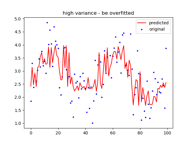
score=model.score(x,y)
print(score)
0.6066306757957185
mse =mean_squared_error(y, pred_y)
print(“Mean Squared Error:”,mse)
Mean Squared Error: 0.30499845231798917
rmse = math.sqrt(mse)
print(“Root Mean Squared Error:”, rmse)
Root Mean Squared Error: 0.5522666496521306
How to Fit Regression Data with CNN Model in Python
https://www.datatechnotes.com/2019/12/how-to-fit-regression-data-with-cnn.html
from sklearn.datasets import load_boston
from keras.models import Sequential
from keras.layers import Dense, Conv1D, Flatten
from sklearn.model_selection import train_test_split
from sklearn.metrics import mean_squared_error
import matplotlib.pyplot as plt
boston = load_boston()
x, y = boston.data, boston.target
print(x.shape)
(506, 13)
An x data has two dimensions that are the number of rows and columns.
Here, we need to add the third dimension that will be the number of the single input row.
x = x.reshape(x.shape[0], x.shape[1], 1)
print(‘Shape with single input row ‘,x.shape)
xtrain, xtest, ytrain, ytest=train_test_split(x, y, test_size=0.15)
model = Sequential()
model.add(Conv1D(32, 2, activation=”relu”, input_shape=(13, 1)))
model.add(Flatten())
model.add(Dense(64, activation=”relu”))
model.add(Dense(1))
model.compile(loss=”mse”, optimizer=”adam”)
model.summary()
Next, we’ll fit the model with train data.
model.fit(xtrain, ytrain, batch_size=12,epochs=200, verbose=0)
ypredtrain = model.predict(xtrain)
print(“MSE Train: %.4f” % mean_squared_error(ytrain, ypredtrain))
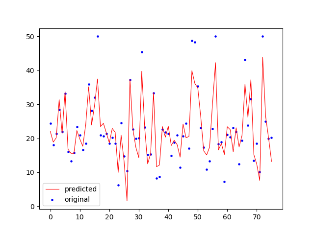
Now we can predict the test data with the trained model.
ypred = model.predict(xtest)
21.21026409947595
print(“MSE Predicts: %.4f” % mean_squared_error(ytest, ypred))
print(‘MSE Evaluate: ‘,model.evaluate(xtest, ytest))
MSE: 19.8953
x_ax = range(len(ypred))
plt.scatter(x_ax, ytest, s=5, color=”blue”, label=”original”)
plt.plot(x_ax, ypred, lw=0.8, color=”red”, label=”predicted”)
plt.legend()
plt.show()
“””
https://medium.com/code-heroku/introduction-to-exploratory-data-analysis-eda-c0257f888676
Here is a quick overview of the things that you are going to learn in this article:
Descriptive Statistics
Grouping of Data
Handling missing values in dataset
ANOVA: Analysis of variance
Correlation
“””
import pandas as pd
import matplotlib.pyplot as plt
import seaborn as sns
import numpy as np
from scipy import stats
df = pd.read_csv(BASEPA+’data/automobile2.csv’) #read data from CSV file
print(df.head())
print(df.describe())
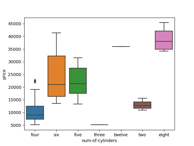
print(df[‘num-of-doors’].value_counts())
sns.boxplot(x=’num-of-cylinders’,y=’price’,data=df)
plt.show()
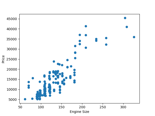
plt.scatter(df[‘engine-size’],df[‘price’])
plt.xlabel(‘Engine Size’)
plt.ylabel(‘Price’)
plt.show()
“””
count,bin_edges = np.histogram(df[‘peak-rpm’])
df[‘peak-rpm’].plot(kind=’hist’,xticks=bin_edges)
plt.xlabel(‘Value of peak rpm’)
plt.ylabel(‘Number of cars’)
plt.grid()
plt.show()
“””
df_temp = df[[‘num-of-doors’,’body-style’,’price’]]
df_group = df_temp.groupby([‘num-of-doors’,’body-style’],as_index=False).mean()
print(df_group)
show missing values
sns.heatmap(df.isnull())
plt.show()
ANOVA is a statistical method which is used for figuring out the relation between different groups of categorical data.
F-test score: It calculates the variation between sample group means divided by variation within sample group.
Correlation is a statistical metric for measuring to what extent different variables are interdependent.
temp_df = df[[‘make’,’price’]].groupby([‘make’])
print(stats.f_oneway(temp_df.get_group(‘audi’)[‘price’],temp_df.get_group(‘volvo’)[‘price’]))
temp_df.plot()
plt.show()
print(stats.f_oneway(temp_df.get_group(‘jaguar’)[‘price’],temp_df.get_group(‘honda’)[‘price’]))
“””
Notice that in this case, we got a very high F-Test score(around 401) with a p value around 1.05 * 10^-11
because, the variance between the average price of “jaguar†and “honda†is huge.
“””
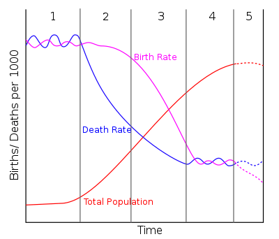
In demography, demographic transition is a phenomenon and theory which refers to the historical shift from high birth rates and high infant death rates in societies with minimal technology, education (especially of women) and economic development, to low birth rates and low death rates in societies with advanced technology, education and economic development, as well as the stages between these two scenarios.
“””
plt.bar(df[‘make’],df[‘price’])
plt.xlabel(‘Maker’)
plt.ylabel(‘Price’)
plt.show()
“””
“””
correlation_matrix = df.corr()
sns.heatmap(correlation_matrix, annot=True)
plt.show()
“””
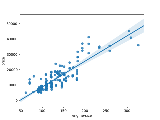
sns.regplot(x=’engine-size’,y=’price’,data=df)
plt.show()
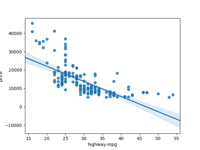
sns.regplot(x=’highway-mpg’,y=’price’,data=df)
plt.show()
if name__ == ‘__main‘:
unittest.main()
ref for remote testing: https://www.javatpoint.com/selenium-python


program Factorial
var Counter, Factorial: integer;
begin
Counter := 5;
Factorial := 1;
while Counter > 0 do begin
Factorial := Factorial * Counter;
Counter := Counter – 1;
end;
Write(Factorial);
end.
LikeLike
Q: “What is the most impressive thing you have seen a software engineer do in an interview?”
A guy wrote some code on a whiteboard and then sat down. Reviewing the code, something didn’t make sense. So, I asked a question about a variable.
Dude says: “Oh, sorry about that.”
Un-caps the whiteboard pen he has in his hand, throws it at the board (like a dart), making a dot between two words. Catches the whiteboard pen as it bounces back, caps it, turns around saying: “That better?”
I looked at it, and I was like: “Yeah.”
LikeLike
Fresh maXbox4:
https://torry.net/files/tools/developers/scripters/maxbox4.zip
LikeLike