
The use of prior time steps to predict the next time step is called the sliding window method. For short, it may be called the window method in some literature. In statistics and time series analysis, this is called a lag or lag method.
The number of previous time steps is called the window width or size of the lag.
This sliding window is the basis for how we can turn any time series dataset into a supervised learning problem. From this simple example, we can notice a few things:
We can see how this can work to turn a time series into either a regression or a classification supervised learning problem for real-valued or labeled time series values.
We can see how once a time series dataset is prepared this way that any of the standard linear and nonlinear machine learning algorithms may be applied, as long as the order of the rows is preserved.

We can see how the width sliding window can be increased to include more previous time steps.
We can see how the sliding window approach can be used on a time series that has more than one value, or so-called multivariate time series.

https://machinelearningmastery.com/time-series-forecasting-supervised-learning/
>>> import pandas_datareader.data as web
>>> df= web.DataReader('^SSMI', data_source='yahoo',start='09-11-2010')
from sklearn.preprocessing import LabelEncoder
labelencoder= LabelEncoder() #initializing an object of class LabelEncoder
data['C'] = labelencoder.fit_transform(data['C']) #fitting and transforming the desired categorical column.
df.loc[(df!=0).any(axis=1)]
df= df[df['ColName'] != 0]
>>> df['Date'] = pd.to_datetime(df.index)
>>> df['Date'] = pd.to_datetime(df.index)
>>> df.info()
Name: day, Length: 1217, dtype: int64
>>> df['weekday'] = pd.DatetimeIndex(df['Date']).weekday
>>> df.corr()
High Low Open ... C day weekday
High 1.000000 0.998770 0.999482 ... 0.976134 -0.020020 0.002322
Low 0.998770 1.000000 0.999033 ... 0.974153 -0.020093 0.001344
Open 0.999482 0.999033 1.000000 ... 0.974553 -0.018877 0.003661
Close 0.999244 0.999400 0.998730 ... 0.975822 -0.020204 0.001031
Volume -0.123889 -0.148456 -0.131867 ... -0.117059 0.015028 0.185688
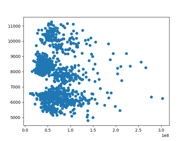
>>> plt.scatter(df.Volume,df.weekday)
<matplotlib.collections.PathCollection object at 0x0000001258226AC8>
>>> plt.show()

import pandas_datareader.data as web
df= web.DataReader('^SSMI', data_source='yahoo',start='09-11-2010')
#quotes = quotes_historical_yahoo_ochl("INTC",
# datetime.date(1994, 4, 5), datetime.date(2015, 7, 3))
quotes = df
print(quotes.info(5))
x_ax_time = range(len(df))
plt.plot(x_ax_time, quotes['Close'])
plt.show()
# Extract the required values
# ValueError: invalid literal for int() with base 10: 'H'
# dates = np.array([quote[0] for quote in quotes], dtype=np.int)
dates = quotes.index
#closing_values = np.array([quote[3] for quote in quotes])
#volume_of_shares = np.array([quote[5] for quote in quotes])[1:]
closing_values = np.array(quotes['Close'])
volume_of_shares = np.array(quotes['Volume'])
# Take diff of closing values and computing rate of change
diff_percentage = 100.0 * np.diff(closing_values) / closing_values[:-1]
dates = dates[1:]
# ValueError: all the input array dimensions for the concatenation axis must match exactly, but along dimension 0,
# the array at index 0 has size 2488 and the array at index 1 has size 2489
# Stack the percentage diff and volume values column-wise for training
Xm = np.column_stack([diff_percentage, volume_of_shares[1:]])
# Create and train Gaussian HMM
print ("\nTraining HMM....& Plot")
hmm_model = GaussianHMM(n_components=3, covariance_type="diag", n_iter=1000)
hmm_model.fit(Xm)
y_pred = hmm_model.predict(Xm)
print("Model Score:", hmm_model.score(Xm))
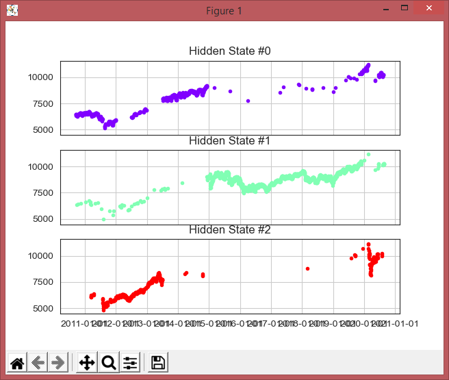
# Plot the in sample hidden states closing values
Xm2 = np.column_stack([diff_percentage[1:], volume_of_shares[2:]])
#hmm_model.fit(Xm2)
plot_in_sample_hidden_states(hmm_model, quotes[2:], Xm2)
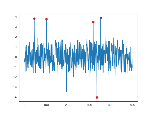
# Generate data using model
# https://www.quantstart.com/articles/market-regime-detection-using-hidden-markov-models-in-qstrader/
num_samples = 500
samples, _ = hmm_model.sample(num_samples)
plt.plot(np.arange(num_samples), samples[:,0], c='black')
plt.show()


 @staticmethod
    def _extract_features(data):
        open_price = np.array(data['open'])
        close_price = np.array(data['close'])
        high_price = np.array(data['high'])
        low_price = np.array(data['low'])

        # Compute fraction change in close, high and low prices
        # which would be used a feature
        frac_change = (close_price - open_price) / open_price
        frac_high = (high_price - open_price) / open_price
        frac_low = (open_price - low_price) / open_price

        return np.column_stack((frac_change,frac_high,frac_low))
        # ret


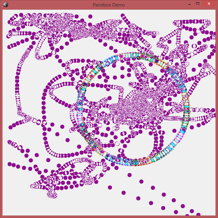


procedure TPaintForm1Timer1Timer(Sender: TObject);
var i : real;
  x1,x2,y1,y2 : integer;
begin
  straal:=straal+3;
  if straal>500 then straal:=0;
  repeat
    r:=r+16;
    if r>255 then
      r:=0;
    g:=g+13;
    if g>255 then
      g:=0;
    b:=b+10;
    if b>255 then
      b:=0;
    i:=i+pi/65;
    x1:=Round(Sin(i)*straal);
    y1:=Round(Cos(i)*straal);
    x2:=Round(Sin(i)*straal+20);
    y2:=Round(Cos(i)*straal+20);
    Paintbox1.Canvas.Pen.Style:=psclear;
    Paintbox1.Canvas.Brush.Color:=RGB(r,g,b);
    Paintbox1.Canvas.Ellipse(400+x1,300+y1,400+x2,300+y2);
  until i>=2*pi;
end;
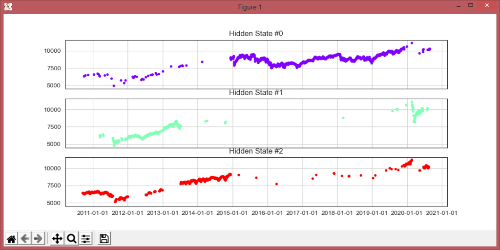
In a Hidden Markov Model (HMM), we have an invisible Markov chain (which we cannot observe), and each state generates in random one out of k observations, which are visible to us. Let’s look at an example of the SMI Chart over 10 years above.
#sign:max: MAXBOX8: 13/03/2019 07:46:37
# optimal moving average OMA for market index signals - max kleiner
import numpy as np
import matplotlib.pyplot as plt
from sklearn import tree
from sklearn.svm import SVC
from sklearn.ensemble import RandomForestClassifier
from sklearn.linear_model import LogisticRegression
from sklearn.metrics import accuracy_score
from sklearn.model_selection import train_test_split
# [volume, weight_index, call_put_ratio]
X = [[181, 80, 44], [177, 70, 43], [160, 60, 38], [154, 54, 37], [166, 65, 40],
[190, 90, 47], [175, 64, 39],
[177, 70, 40], [159, 55, 37], [171, 75, 42], [181, 85, 43], [168, 75, 41], [168, 77, 41]]
Y = ['buy', 'buy', 'sell', 'sell', 'buy', 'buy', 'sell', 'sell',
'sell', 'buy', 'buy', 'sell', 'sell']
test_data = [[190, 70, 43],[154, 75, 42],[181,65,40]]
test_labels = ['buy','buy','buy']
#DecisionTreeClassifier
dtc_clf = tree.DecisionTreeClassifier()
dtc_clf = dtc_clf.fit(X,Y)
dtc_prediction = dtc_clf.predict(test_data)
print (dtc_prediction)
#RandomForestClassifier
rfc_clf = RandomForestClassifier()
rfc_clf.fit(X,Y)
rfc_prediction = rfc_clf.predict(test_data)
print (rfc_prediction)
#Support Vector Classifier
s_clf = SVC(gamma='auto', C=0.1, kernel='linear')
s_clf.fit(X,Y)
s_prediction = s_clf.predict(test_data)
print (s_prediction)
#LogisticRegression
l_clf = LogisticRegression(solver='liblinear')
l_clf.fit(X,Y)
l_prediction = l_clf.predict(test_data)
print (l_prediction)
#accuracy scores
dtc_tree_acc = accuracy_score(dtc_prediction,test_labels)
rfc_acc = accuracy_score(rfc_prediction,test_labels)
l_acc = accuracy_score(l_prediction,test_labels)
s_acc = accuracy_score(s_prediction,test_labels)
classifiers = ['Decision Tree', 'Random Forest', 'Logistic Regression' , 'SVC']
accuracy = np.array([dtc_tree_acc, rfc_acc, l_acc, s_acc])
max_acc = np.argmax(accuracy)
print(classifiers[max_acc] + ' is the best classifier for this problem')
print(dtc_tree_acc, rfc_acc, l_acc,s_acc)
# Get quotes from Yahoo finance and find optimal moving average
import pandas_datareader.data as web
df= web.DataReader('^SSMI', data_source='yahoo',start='09-11-2010')
#DataMax - Predict for 30 days; Predicted has the data of Adj. Close shifted up by 30 rows
forecast_len=60 #oma is 5
quotes = df
print(quotes.info(5))
df['_SMI_20'] = df.iloc[:,3].rolling(window=20).mean()
df['_SMI_60'] = df.iloc[:,3].rolling(window=forecast_len).mean()
df['_SMI_180'] = df.iloc[:,3].rolling(window=160).mean()
x_ax_time = quotes.index #range(len(df))
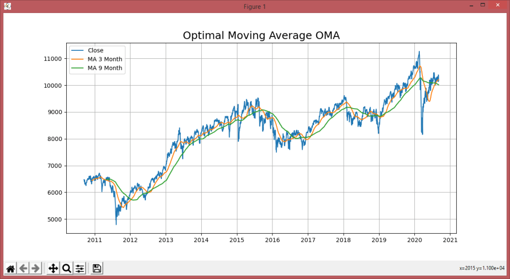
plt.figure(figsize=[12,8])
plt.grid(True)
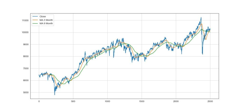
plt.title('Optimal Moving Average OMA', fontsize=18)
plt.plot(x_ax_time, quotes['Close'], label='Close')
plt.plot(x_ax_time, df['_SMI_60'],label='MA 3 Month')
plt.plot(x_ax_time, df['_SMI_180'],label='MA 9 Month')
#plt.xlabel('days', fontsize=15)
# plt.plot_date(quotes.index, quotes['Close'])
plt.legend(loc=2)
plt.show()
dates = quotes.index
dates = dates[1:]
#closing_values = np.array([quote[3] for quote in quotes])
#volume_of_shares = np.array([quote[5] for quote in quotes])[1:]
closing_values = np.array(quotes['Close'])
volume_of_shares = np.array(quotes['Volume'])
#Predict for 30 days; Predicted has the data of Close shifted up by 30 rows
ytarget = quotes['Close'].shift(-forecast_len)
ytarget= ytarget[:-forecast_len]
Xdata= closing_values[:-forecast_len]
from sklearn.svm import SVR
# Split datasets into training and test sets (80% and 20%)
print('shape len2: ',len(ytarget),len(Xdata))
x_train,x_test,y_train,y_test=train_test_split(Xdata,ytarget,test_size=0.2, \ random_state= 72)
print('shape len3: ',len(x_train),len(y_train))
# - Create SVR model and train it
svr_rbf=SVR(kernel='rbf',C=1e3,gamma=0.1)
x_train = x_train.reshape(-1,1)
svr_rbf.fit(x_train,y_train)
#DBASTAr - Get score
svr_rbf_confidence=svr_rbf.score(x_test.reshape(-1,1),y_test)
print(f"SVR Confidence: {round(svr_rbf_confidence*100,2)}%")
"""" Column Non-Null Count Dtype
--- ------ -------------- -----
0 High 2500 non-null float64
1 Low 2500 non-null float64
2 Open 2500 non-null float64
3 Close 2500 non-null float64
4 Volume 2500 non-null int64
5 Adj Close 2500 non-null float64
dtypes: float64(5), int64(1)
memory usage: 136.7 KB
"""

#sign:max: MAXBOX8: 07/09/2020 07:46:37
# optimal moving average OMA for market index signals - max kleiner
# v2 shell argument forecast days - 4 lines compare - ^GDAXI for DAX
# pip install pandas-datareader
import numpy as np
import matplotlib.pyplot as plt
import sys
from sklearn import tree
from sklearn.svm import SVC
from sklearn.ensemble import RandomForestClassifier
from sklearn.linear_model import LogisticRegression
from sklearn.preprocessing import StandardScaler
from sklearn.metrics import accuracy_score
from sklearn.model_selection import train_test_split
# [volume, weight_index, call_put_ratio]
X = [[181, 80, 44],[177, 70, 43],[160, 60, 38],[154, 54, 37],[166, 65, 40],
[190, 90, 47],[175, 64, 39],
[177, 70, 40],[159, 55, 37],[171, 75, 42],[181, 85, 43],[168, 75, 41],[168, 77, 41]]
Y = ['buy', 'buy', 'sell', 'sell', 'buy', 'buy', 'sell', 'sell',
'sell', 'buy', 'buy', 'sell', 'sell']
test_data = [[190, 70, 43],[154, 75, 42],[181,65,40]]
test_labels = ['buy','buy','buy']
#DecisionTreeClassifier
dtc_clf = tree.DecisionTreeClassifier()
dtc_clf = dtc_clf.fit(X,Y)
dtc_prediction = dtc_clf.predict(test_data)
print (dtc_prediction)
#RandomForestClassifier
rfc_clf = RandomForestClassifier()
rfc_clf.fit(X,Y)
rfc_prediction = rfc_clf.predict(test_data)
print (rfc_prediction)
#Support Vector Classifier
s_clf = SVC(gamma='auto', C=0.1, kernel='linear')
s_clf.fit(X,Y)
s_prediction = s_clf.predict(test_data)
print (s_prediction)
#LogisticRegression
l_clf = LogisticRegression(solver='liblinear')
l_clf.fit(X,Y)
l_prediction = l_clf.predict(test_data)
print (l_prediction)
#accuracy scores
dtc_tree_acc = accuracy_score(dtc_prediction,test_labels)
rfc_acc = accuracy_score(rfc_prediction,test_labels)
l_acc = accuracy_score(l_prediction,test_labels)
s_acc = accuracy_score(s_prediction,test_labels)
classifiers = ['Decision Tree', 'Random Forest', 'Logistic Regression' , 'SVC']
accuracy = np.array([dtc_tree_acc, rfc_acc, l_acc, s_acc])
max_acc = np.argmax(accuracy)
print(classifiers[max_acc] + ' is the best classifier for this problem')
print(dtc_tree_acc, rfc_acc, l_acc,s_acc)
# Quotes from Yahoo finance and find optimal moving average
import pandas_datareader.data as web
#DataMax - Predict for 30 days; Predicted has the data of Adj. Close shifted up by 30 rows
forecast_len=80 #default oma is 5
YQUOTES = '^SSMI'
PLOT = 'Y'
try:
forecast_len = int(sys.argv[1])
#forecast_len= int(' '.join(sys.argv[1:]))
YQUOTES = str(sys.argv[2])
PLOT = str(sys.argv[3])
except:
forecast_len= forecast_len
YQUOTES = YQUOTES
#YQUOTES = 'BTC-USD' #^GDAXI' , '^SSMI' , '^GSPC' (S&P 500 ) - ticker='GOOGL'
try:
df= web.DataReader(YQUOTES, data_source='yahoo',start='09-11-2010')
except:
YQUOTES = '^SSMI'
df= web.DataReader(YQUOTES, data_source='yahoo',start='09-11-2010')
print('Invalid Quote Symbol got ^SSMI instead')
#data = ' '.join(sys.argv[1:])
print ('get forecast len:',forecast_len, 'for ', YQUOTES)
quotes = df
print(quotes.info(5))
print(quotes['Close'][:5])
print(quotes['Close'][-3:])
df['_SMI_20'] = df.iloc[:,3].rolling(window=20).mean()
df['_SMI_60'] = df.iloc[:,3].rolling(window=60).mean()
df['_SMI_180'] = df.iloc[:,3].rolling(window=180).mean()
df['_SMI_OMA'] = df.iloc[:,3].rolling(window=forecast_len).mean()
#"""
if PLOT=='Y':
x_ax_time = quotes.index #range(len(df))
plt.figure(figsize=[12,7])
plt.grid(True)
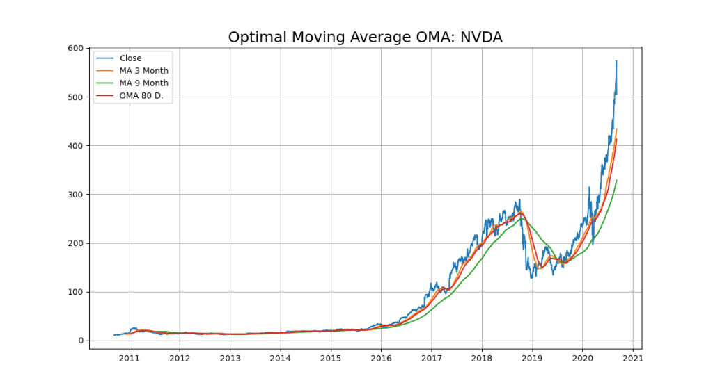
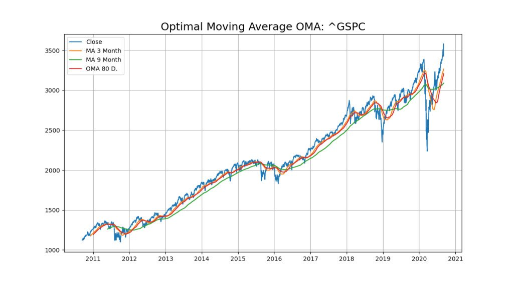
plt.title('Optimal Moving Average OMA: '+YQUOTES, fontsize=18)
plt.plot(x_ax_time, quotes['Close'], label='Close')
plt.plot(x_ax_time, df['_SMI_60'],label='MA 3 Month')
plt.plot(x_ax_time, df['_SMI_180'],label='MA 9 Month')
plt.plot(x_ax_time, df['_SMI_OMA'],label='OMA '+str(forecast_len)+' D.')
#plt.xlabel('days', fontsize=15)
# plt.plot_date(quotes.index, quotes['Close'])
plt.legend(loc=2)
plt.show()
#"""
dates = quotes.index
dates = dates[1:]
#closing_values = np.array([quote[3] for quote in quotes])
#volume_of_shares = np.array([quote[5] for quote in quotes])[1:]
closing_values = np.array(quotes['Close'])
volume_of_shares = np.array(quotes['Volume'])
#Predict for 30 days; Predicted has the Quotes of Close shifted up by 30 rows
ytarget= quotes['Close'].shift(-forecast_len)
ytarget= ytarget[:-forecast_len]
Xdata= closing_values[:-forecast_len]
#print('Offset shift:',ytarget[:10])
# Feature Scaling
#sc_X = StandardScaler()
#sc_y = StandardScaler()
#Xdata = sc_X.fit_transform(Xdata.reshape(-1,1))
#You need to do this is that pandas Series objects are by design one dimensional.
#ytarget = sc_y.fit_transform(ytarget.values.reshape(-1,1))
from sklearn.svm import SVR
# Split datasets into training and test sets (80% and 20%)
print('target shape len2: ',len(ytarget),len(Xdata))
x_train,x_test,y_train,y_test=train_test_split(Xdata,ytarget,test_size=0.2, \
random_state= 72)
print('xtrain shape len3: ',len(x_train),len(y_train))
# - Create SVR model and train it
svr_rbf= SVR(kernel='rbf',C=1e3,gamma=0.1)
x_train = x_train.reshape(-1,1)
svr_rbf.fit(x_train,y_train)
# Predicting single value as new result
print('predict old in :', forecast_len, svr_rbf.predict([quotes['Close'][:1]]))
print('predict now in :', forecast_len, svr_rbf.predict([quotes['Close'][-1:]]))
#DBASTAr - Get score
svr_rbf_confidence=svr_rbf.score(x_test.reshape(-1,1),y_test)
print(f"SVR Confidence: {round(svr_rbf_confidence*100,2)}%")
"""" Column Non-Null Count Dtype
--- ------ -------------- -----
0 High 2500 non-null float64
1 Low 2500 non-null float64
2 Open 2500 non-null float64
3 Close 2500 non-null float64
4 Volume 2500 non-null int64
5 Adj Close 2500 non-null float64
dtypes: float64(5), int64(1)
memory usage: 136.7 KB
df.index = pd.to_datetime(df.index)
"""
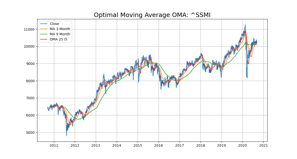
So I had to find out the optimal moving average within a loop from about 20 to 50 days to get a high confidence score in steps of 5 days interval:
memory usage: 137.1 KB
None
Date
2010-09-13 6471.770020
2010-09-14 6466.319824
2010-09-15 6434.009766
2010-09-16 6424.160156
2010-09-17 6389.020020
Name: Close, dtype: float64
Date
2020-09-04 10153.089844
2020-09-07 10297.799805
2020-09-08 10261.019531
Name: Close, dtype: float64
target shape len2: 2457 2457
xtrain shape len3: 1965 1965
predict old in : 50 [6532.54014764]
predict now in : 50 [8599.34565955]
SVR Confidence: 68.28%
Serie 50 : 68.28%
List of 20-50 days so according to the score 25 days would be best:
20 – 69.05%
25 – 70.04%
30 – 67.8%
35 – 67.04%
40 – 67.74%
45 – 68.07%
50 – 68.28%
begin //@main

  saveString(exepath+'mygauss.py',ACTIVESCRIPT);
  sleep(200)
  //if fileExists(PYPATH+'python.exe') then
   if fileExists(PYSCRIPT) then begin

     //ShellExecute3('cmd','/k '+PYPATH+'python.exe '+PYCode+ ' '+
     //                       PYFILE ,secmdopen);
     //ShellExecute3('cmd','/k '+PYPATH+'python.exe && '+PYFILE +'&& mygauss3()'
     //                                  ,secmdopen);
      { ShellExecute3('cmd','/k '+PYPATH+
                        'python.exe && exec(open('+exepath+'mygauss.py'').read())'
                        ,secmdopen);
                 }

     { ShellExecute3('cmd','/k '+PYPATH+
                        'python.exe '+exepath+'mygauss.py', secmdopen); }
     // ShellExecute3(PYPATH+'python.exe ',exepath+'mygauss.py'
     //                   ,secmdopen);
     maxform1.console1click(self);
     memo2.height:= 205;
     // maxform1.shellstyle1click(self);
     // writeln(GetDosOutput(PYPATH+'python.exe '+PYSCRIPT,'C:\'));
    fcast:= 75;
    olist:= TStringlist.create;
    GetDosOutput('py '+PYSCRIPT+' '+itoa(fcast)+' "^SSMI" "Y"','C:\');
    for it:= 20 to 50 do
       if it mod 5=0 then begin
         //writeln(GetDosOutput('py '+PYSCRIPT+' '+itoa(it)+' "BTC-USD"'+ ' N','C:\'));
         dosout:= GetDosOutput('py '+PYSCRIPT+' '+itoa(it)+' "^SSMI" "N"','C:\');
         writeln(dosout)
         with TRegExpr.Create do begin
            Expression:=('SVR Confidence: ([0-9\.%]+).*');
            if Exec(dosout) then begin
              PrintF('Serie %d  : %s', [it, Match[1]]);
              olist.add(itoa(it) + ' - '+Match[1])
            end;
          Free;
         end;
       end;
     writeln(olist.text)
     olist.Free;
     // writeln(GetDosOutput('dir *.*','C:\'));
   end;
End.
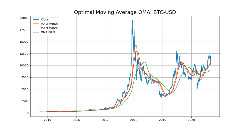
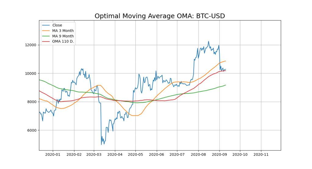
A Use Case with the OMA Model and Bitcoin. Lets find the Opimal Moving Average with a SVR (Epsilon-Support Vector Regression).
The free parameters in the model are C and epsilon.
The implementation is based on libsvm. The fit time complexity is more than quadratic with the number of samples which makes it hard to scale to datasets with more than a couple of 10000 samples (we do have 2185 entries).
Get forecast len: from 20 to 130 for BTC-USD
DatetimeIndex: 2185 entries, 2014-09-16 to 2020-09-10
Data columns (total 6 columns):
# Column Non-Null Count Dtype
— —— ————– —–
0 High 2185 non-null float64
1 Low 2185 non-null float64
2 Open 2185 non-null float64
3 Close 2185 non-null float64
4 Volume 2185 non-null float64
5 Adj Close 2185 non-null float64
dtypes: float64(6)
memory usage: 119.5 KB
None
Date
2014-09-16 457.334015
2014-09-17 424.440002
2014-09-18 394.795990
2014-09-19 408.903992
2014-09-20 398.821014
Name: Close, dtype: float64
Date
2020-09-07 10131.516602
2020-09-08 10242.347656
2020-09-10 10296.268555
Name: Close, dtype: float64
target shape len2: 2055 2055
xtrain shape len3: 1644 1644
predict old in : 130 [596.1518452]
predict now in : 130 [5843.31880494]
SVR Confidence: 59.75%
We loop from 20 to 130 to find the max confidence score:
   QuoteSymbol:= 'BTC-USD'; //'BTC-USD'; //^SSMI    TSLA
    olist:= TStringlist.create;
    olist.NameValueSeparator:= '=';
    //olist.Sorted:= True;
    //olist.CustomSort(@CompareFileName)
    //GetDosOutput('py '+PYSCRIPT+' '+itoa(fcast)+' '+QuoteSymbol+' "Y"','C:\');
    GetDosOutput('py '+RUNSCRIPT+' '+itoa(fcast)+' '+QuoteSymbol+' "Y"','C:\');

    for it:= 20 to 130 do
       if it mod 5=0 then begin
         //(GetDosOutput('py '+PYSCRIPT+' '+itoa(it)+' "BTC-USD"'+ 'Plot?','C:\'));
         dosout:= GetDosOutput('py '+RUNSCRIPT+' '+itoa(it)+' '+QuoteSymbol+' "N"','C:\');
         writeln(dosout)
         with TRegExpr.Create do begin
            //Expression:=('SVR Confidence: ([0-9\.%]+).*');
            Expression:=('SVR Confidence: ([0-9\.]+).*');
            if Exec(dosout) then begin
              PrintF('Serie %d  : %s',[it, Match[1]]);
              olist.add(Match[1]+'='+itoa(it));
              Yvalfloat[it]:= strtofloat(Copy(match[1],1,5));
              //MaxFloatArray
            end;
          Free;
         end;
       end;
     writeln(CR+LF+olist.text)
     writeln('OMA from key value list2: '+floattostr(MaxFloatArray(Yvalfloat)))
     TheMaxOMA:= olist.Values[floattostr(MaxFloatArray(Yvalfloat))];
     writeln('OMA for Chart Signal: '+TheMaxOMA);
     olist.Free;
    (GetDosOutput('py '+RUNSCRIPT+' '+(TheMaxOMA)+' '+QuoteSymbol+' "Y"','C:\'));
   end;
56.9=20
59.04=25
55.73=30
55.86=35
56.87=40
57.71=45
54.23=50
57.08=55
59.64=60
52.66=65
56.68=70
57.06=75
59.75=80
55.68=85
60.32=90
59.43=95
61.42=100
58.69=105
65.31=110
62.47=115
61.89=120
62.35=125
59.75=130
OMA from key value list2: 65.31
OMA for Chart Signal: 110

So the close line (blue) cuts the OMA (redline) from up to down and thats our next sell-signal:

Hidden Markov Models are based on a set of unobserved underlying states amongst which transitions can occur and each state is associated with a set of possible observations. The stock market can also be seen in a similar manner. The underlying states, which determine the behavior of the stock value, are usually invisible to the investor.
LikeLike
Isn’t is a problem as a false condition to use close price as part of one feature:
frac_change = (close_price – open_price) / open_price
and then use the target itself as close price (self similiar)
https://rubikscode.net/2018/10/29/stock-price-prediction-using-hidden-markov-model/
LikeLike
A moving average, also called a rolling or running average, is used to analyze the time-series data by calculating averages of different subsets of the complete dataset. Since it involves taking the average of the dataset over time, it is also called a moving mean (MM) or rolling mean.
https://www.datacamp.com/community/tutorials/moving-averages-in-pandas
LikeLike
DatetimeIndex: 2505 entries, 2010-09-13 to 2020-09-04
Data columns (total 6 columns):
# Column Non-Null Count Dtype
— —— ————– —–
0 High 2505 non-null float64
1 Low 2505 non-null float64
2 Open 2505 non-null float64
3 Close 2505 non-null float64
4 Volume 2505 non-null int64
5 Adj Close 2505 non-null float64
dtypes: float64(5), int64(1)
memory usage: 137.0 KB
None
shape len2: 2445 2445
shape len3: 1956 1956
SVR Confidence: 66.33%
C:\maXbox\mX46210\DataScience\confusionlist>
LikeLike
SVR Confidence: 49.51%
Serie SMI 20-150 : last 49.51%
20 – 69.05%
25 – 70.04%
30 – 67.8%
35 – 67.04%
40 – 67.74%
45 – 68.07%
50 – 68.28%
55 – 67.77%
60 – 64.36%
65 – 64.94%
70 – 67.79%
75 – 65.57%
80 – 64.99%
85 – 62.59%
90 – 64.53%
95 – 61.77%
100 – 59.99%
105 – 57.67%
110 – 55.67%
115 – 58.96%
120 – 55.95%
125 – 53.18%
130 – 53.82%
135 – 54.17%
140 – 55.14%
145 – 52.75%
150 – 49.51%
LikeLike